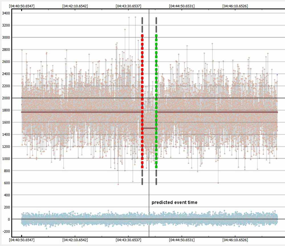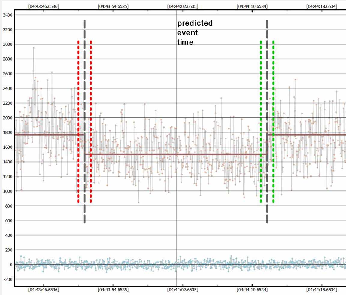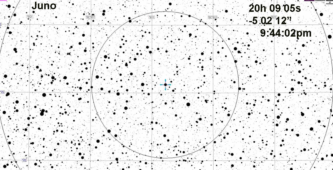
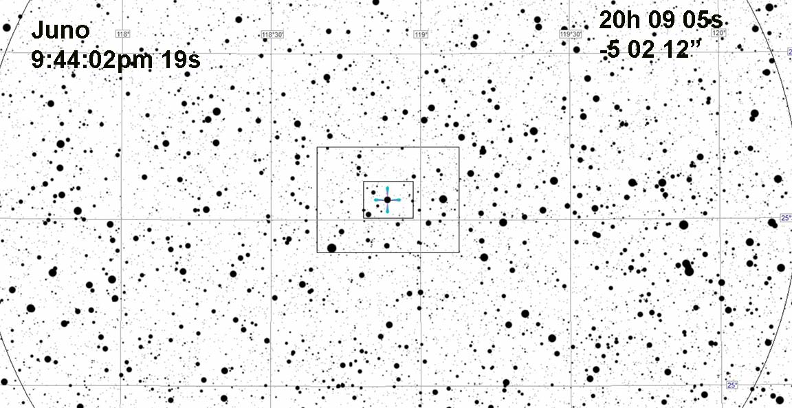
This is a very bright event, but shallow drop of 0.22mag. I'd recommend it at 1x to maximize the number of points, help on saturation. Will want to dial down Gain from 41 normal maximum to something smaller. Duration is 19s. Got to confess there's little scientific value to this one. We have photo'd this one up close and know it well. Any moons probably would have been seen by now. But it's good practice for shallow drop events.
Alt=29, Az=122 in Aquila
|
|
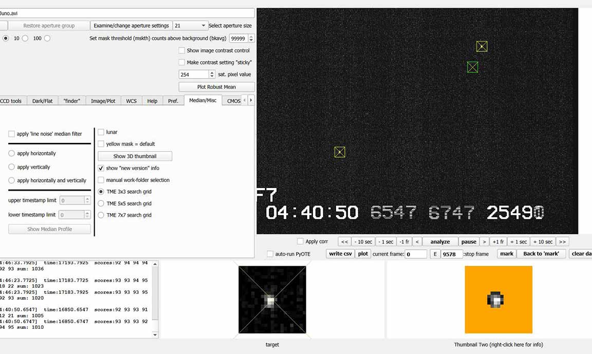
I recorded it for 3 min before and 3 min after the event. I did it at 1x, from driveway, and lowered the computer brightness and also the gain, gain=36. I cut the brightnesss on the IOTA VC 2.4 menu and also the contrast. The star looked bright, but I figured saturation would only affect occasional pixels.
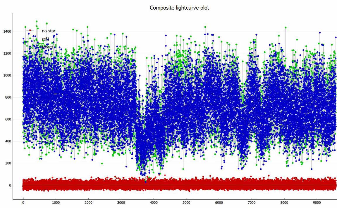
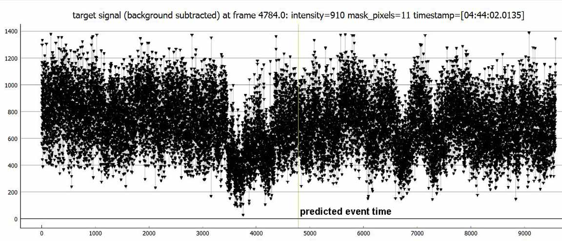
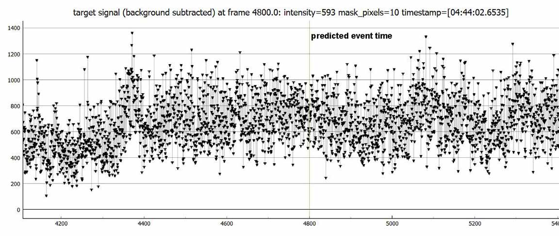
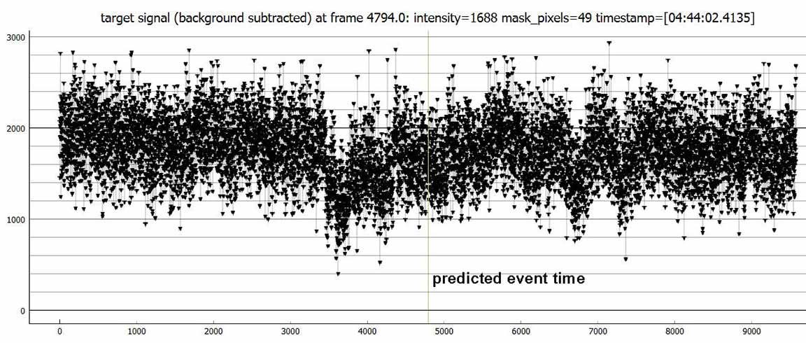
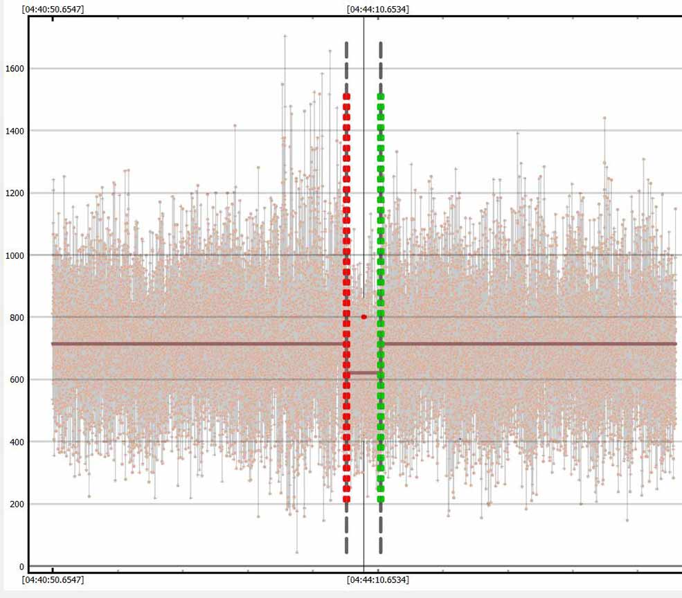
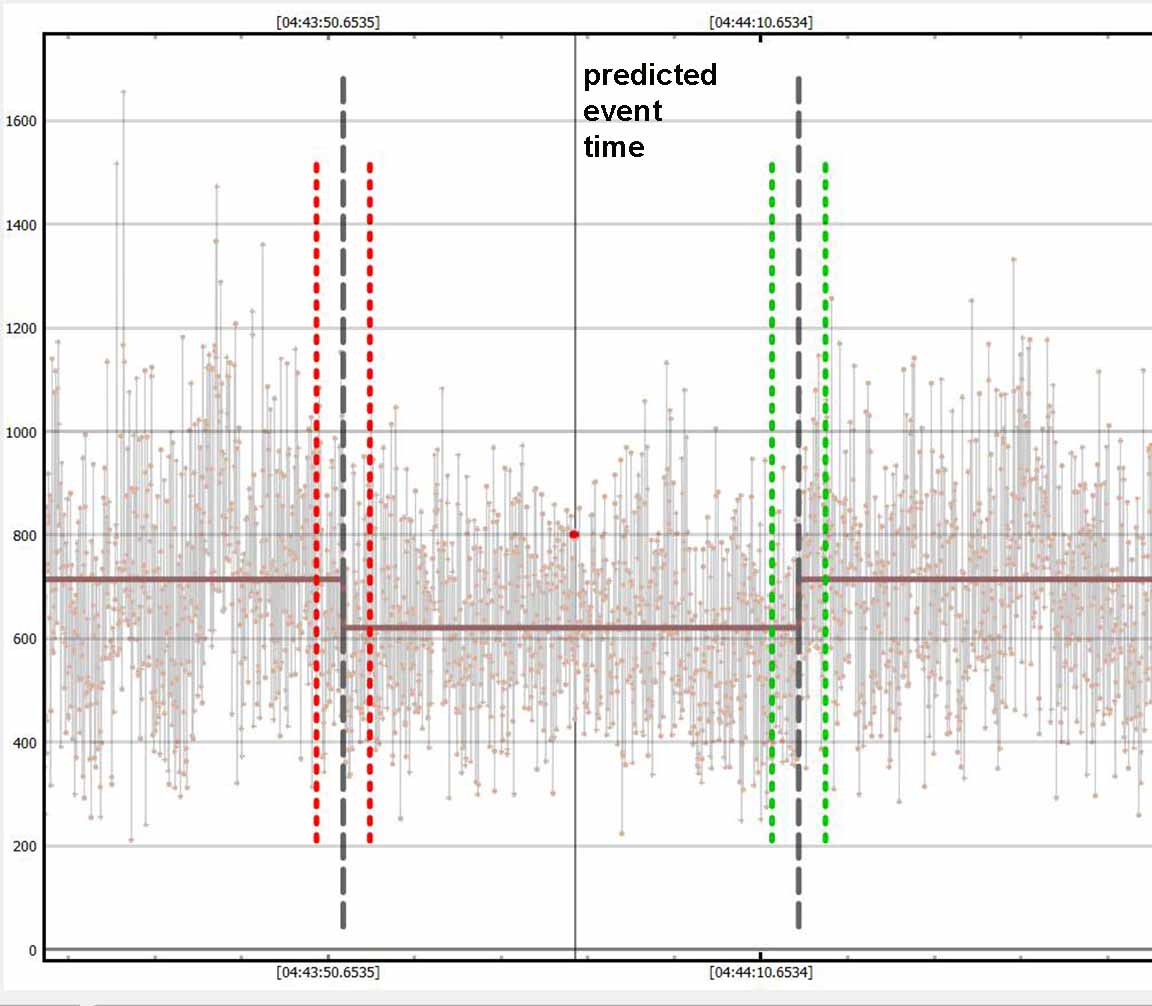
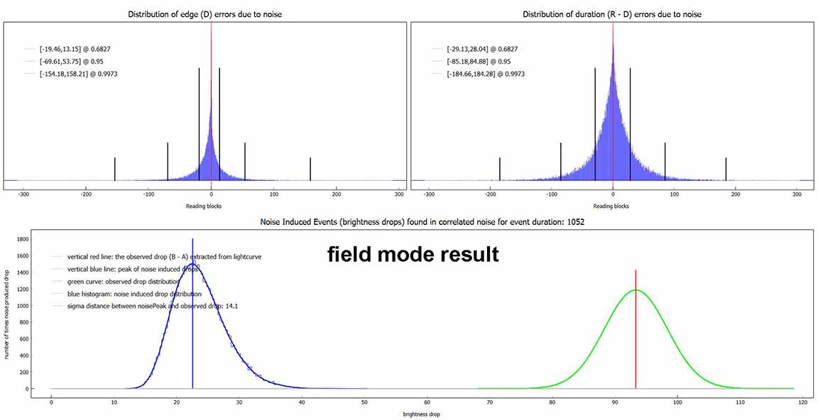
There was evidently more variable aerosol or perhaps poor tracking than I expected. The noise was pretty much corrected for by the reference star, but I'm tempted to re-analyze it with a larger mask and combine fields (not analyze in field mode). I have not done that for the timings below. I set the D and R intervals by eye, to avoid false positives due to remaining noise. I've noticed that even when setting the D and R intervals, PyOTE can still make up its own mind on where it finds the best event. In this case, however, with multiple trials, it always settled on the correct range and the predicted moment was right in the center of the detected 21s occultation.
NIE Test: 14.1 sigma
magDrop report: percentDrop: 13.1 magDrop: 0.152 +/- 0.017 (0.95 ci)
DNR: 0.50
D time: [04:43:51.3535]
D: 0.6800 containment intervals: {+/- 0.3261} seconds
D: 0.9500 containment intervals: {+/- 1.2336} seconds
D: 0.9973 containment intervals: {+/- 3.1239} seconds
R time: [04:44:12.3934]
R: 0.6800 containment intervals: {+/- 0.3261} seconds
R: 0.9500 containment intervals: {+/- 1.2336} seconds
R: 0.9973 containment intervals: {+/- 3.1239} seconds
Duration (R - D): 21.0399 seconds
Duration: 0.6800 containment intervals: {+/- 0.5717} seconds
Duration: 0.9500 containment intervals: {+/- 1.7006} seconds
Duration: 0.9973 containment intervals: {+/- 3.6894} seconds
 |
variable transparency is a bit of a problem in my site this time. |
This variable transparency makes the actual occultation un-noticed |
Even zoomed in, without using the reference star, the occultation is invisible. PyOTE saved the day by allowing calibration, and the occultation is clear in the PyOTE light curves. |
 |
 |
 |
Analysis #2: Bigger 4px mask and use 2x, combining the fields into their frames.
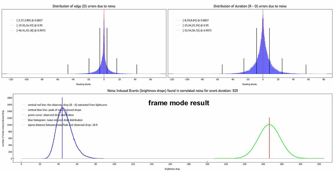
I then re-did the reduction. In PyMovie I let it group fields into frames - no "analyze in field mode" - and I raised the mask size to 4px instead of 2.4px, since the sky was rather dark and the target quite bright, there was little danger of sky noise being a worry, and the advantage is that I could be more certain all the target photons were counted. The result was clearly better. After minimizing the metric interval (chosen to be the entire light curve) in both smoothing length and time offset, the occultation stood out more clearly. The D and R timings had much smaller error bands, most important.
magDrop report: percentDrop: 15.1 magDrop: 0.178 +/- 0.017 (0.95 ci)
DNR: 0.86
D time: [04:43:51.3735]
D: 0.6800 containment intervals: {+/- 0.1852} seconds
D: 0.9500 containment intervals: {+/- 0.7146} seconds
D: 0.9973 containment intervals: {+/- 1.7718} seconds
R time: [04:44:12.3734]
R: 0.6800 containment intervals: {+/- 0.1852} seconds
R: 0.9500 containment intervals: {+/- 0.7146} seconds
R: 0.9973 containment intervals: {+/- 1.7718} seconds
Duration (R - D): 20.9999 seconds
Duration: 0.6800 containment intervals: {+/- 0.3387} seconds
Duration: 0.9500 containment intervals: {+/- 1.0076} seconds
Duration: 0.9973 containment intervals: {+/- 2.2053} seconds
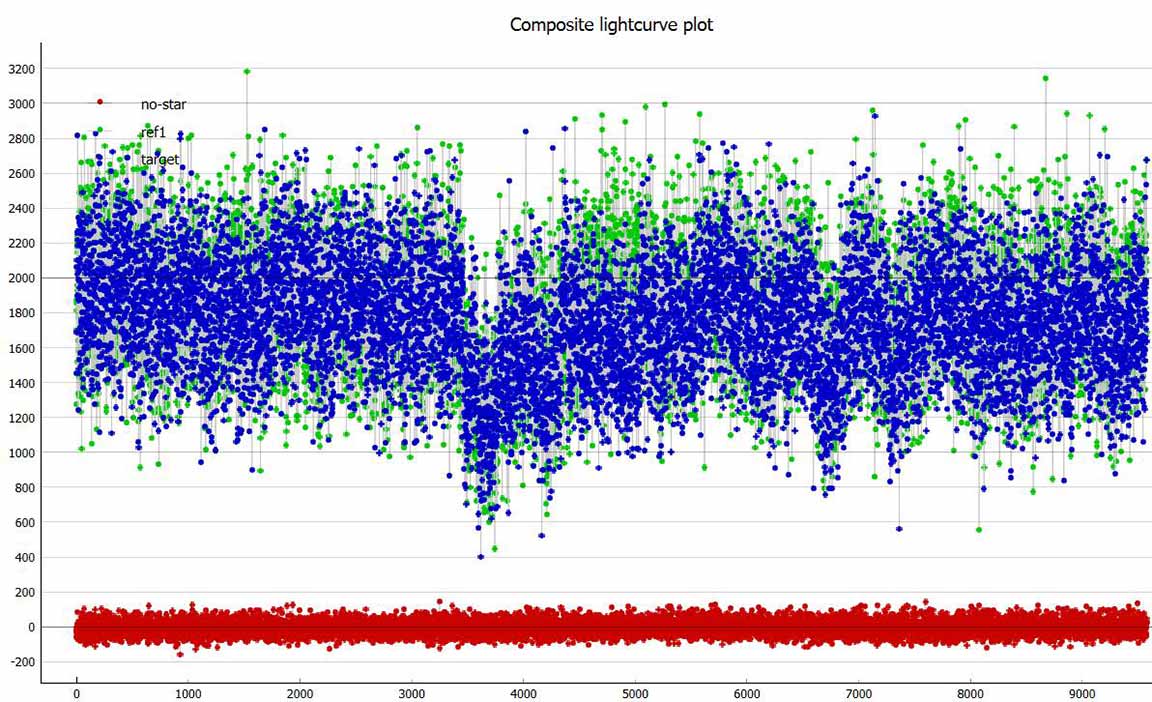 |
Without the reference star, identifying the occultation would have been impossible. |
Better confinement throughout the light curve, makes the shallow but long integration fairly straightforward to see by eye. |
This second analysis provided significantly tighter error baands on the timings. Still the same D and R and duration as the first analysis. |
NIE test was better too; 18.9 sigma instead of 14.1 sigma with the 1x and smaller mask analysis |
Observed from home and got a recording at 1x.
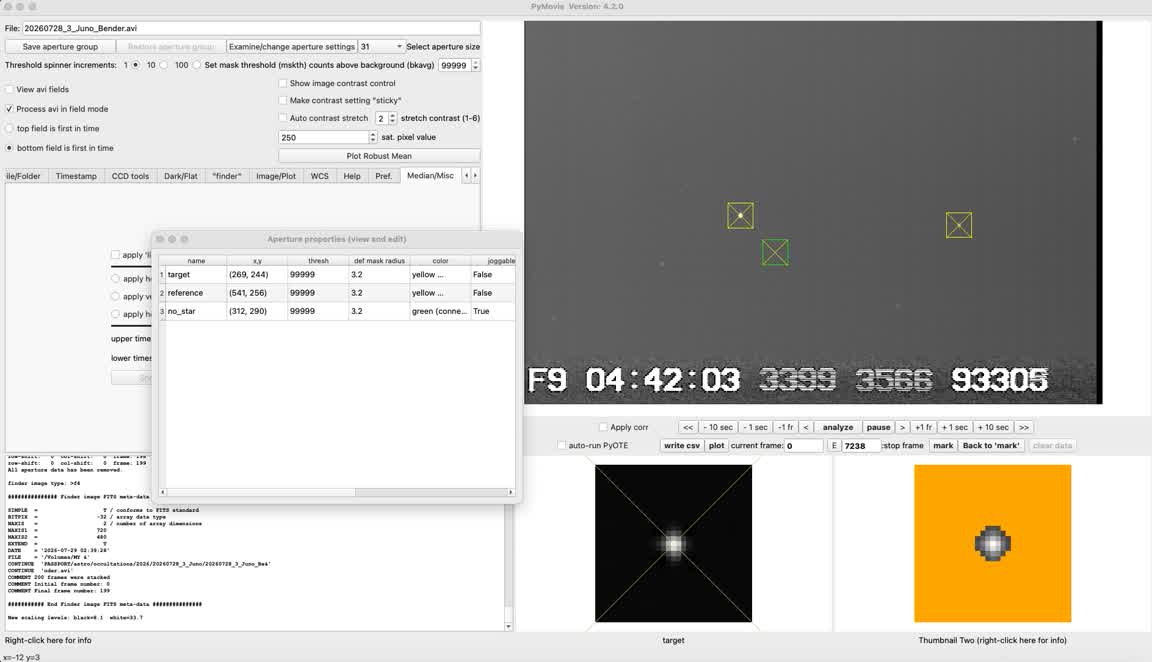
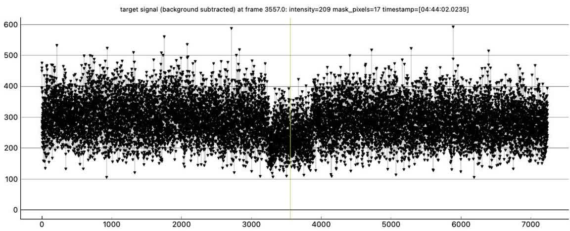
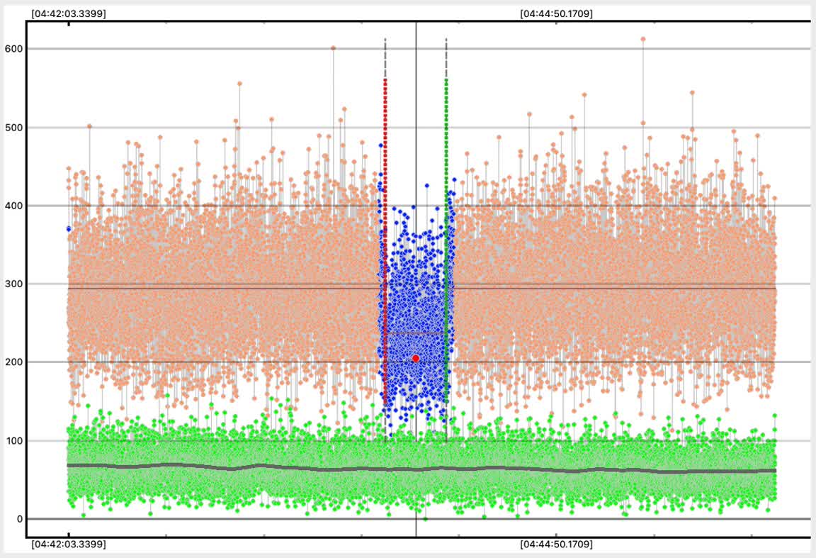
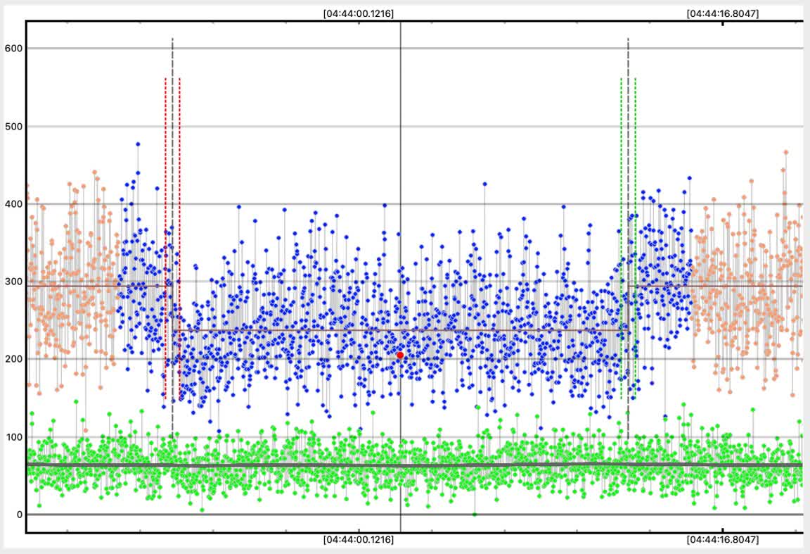
I got a 20.8706s event for Juno, 1x from home. I turned the gain down to 31 to avoid saturation. There was only one other star bright enough for tracking, so I used both the target and the other star for tracking, and used a size 3.2 mask.
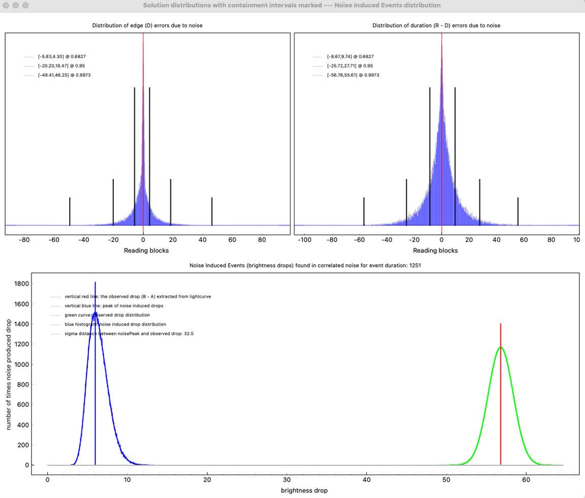
PyOTE NIE sigma distance = 32.5
magDrop report: percentDrop: 19.3 magDrop: 0.233 +/- 0.014 (0.95 ci)
DNR: 0.94
D time: [04:43:51.5965]
D: 0.6800 containment intervals: {+/- 0.0845} seconds
D: 0.9500 containment intervals: {+/- 0.3225} seconds
D: 0.9973 containment intervals: {+/- 0.7980} seconds
R time: [04:44:12.4671]
R: 0.6800 containment intervals: {+/- 0.0845} seconds
R: 0.9500 containment intervals: {+/- 0.3225} seconds
R: 0.9973 containment intervals: {+/- 0.7980} seconds
Duration (R - D): 20.8706 seconds
Duration: 0.6800 containment intervals: {+/- 0.1536} seconds
Duration: 0.9500 containment intervals: {+/- 0.4457} seconds
Duration: 0.9973 containment intervals: {+/- 0.9374} seconds
 |
 |
 |
 |
 |
 |
recorded at 1x, but reduced in PyMovie at 2x since "process in field mode" was left unchecked. The timings below may have to be changed.
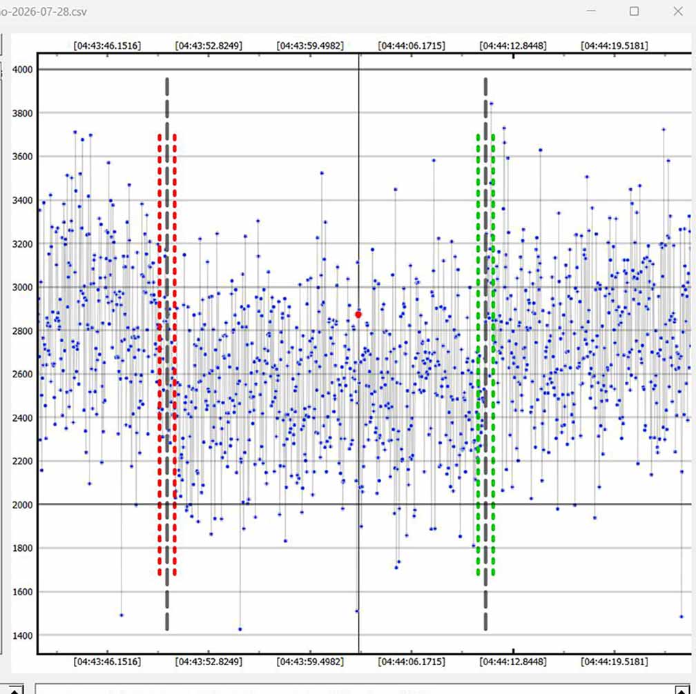
magDrop report: percentDrop: 11.2 magDrop: 0.129 +/- 0.011 (0.95 ci)
 |
 |
 |
 |
 |
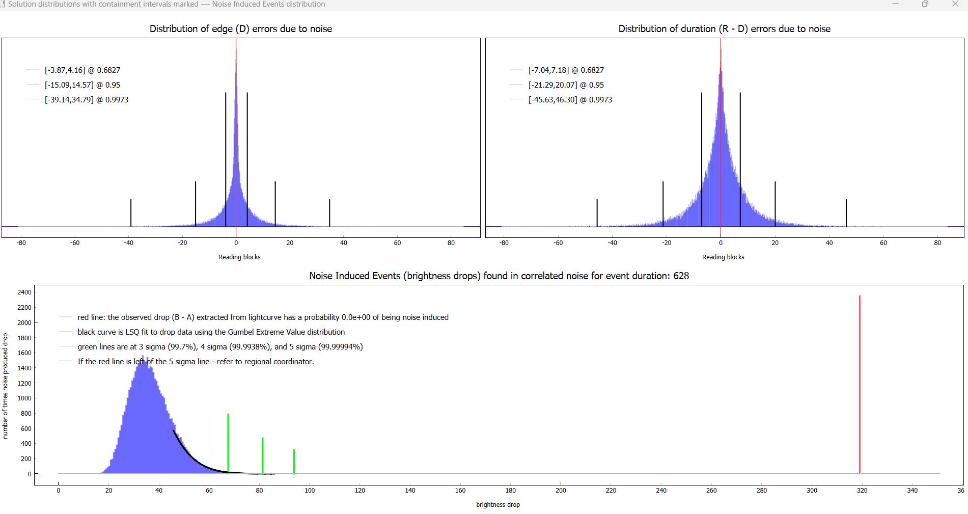 |
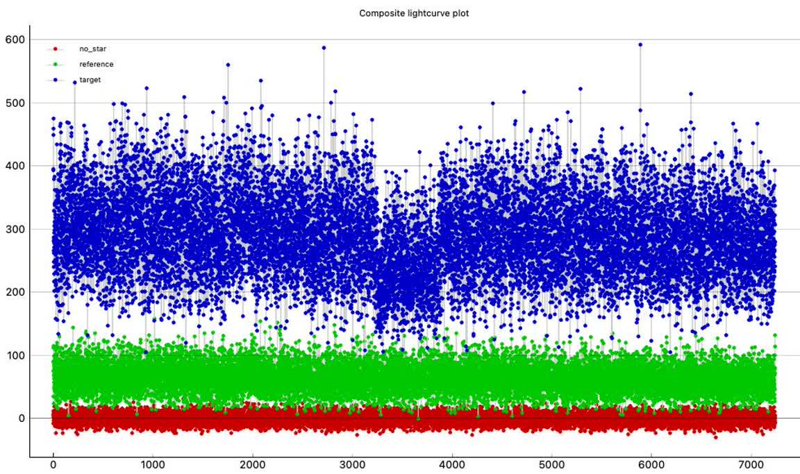
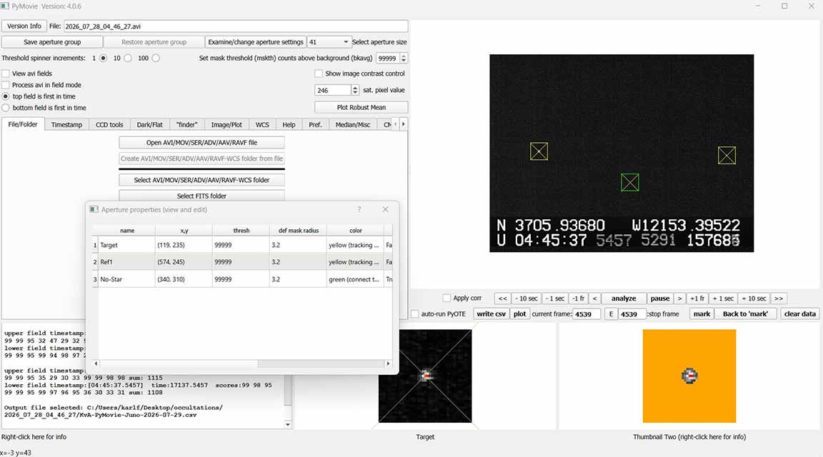
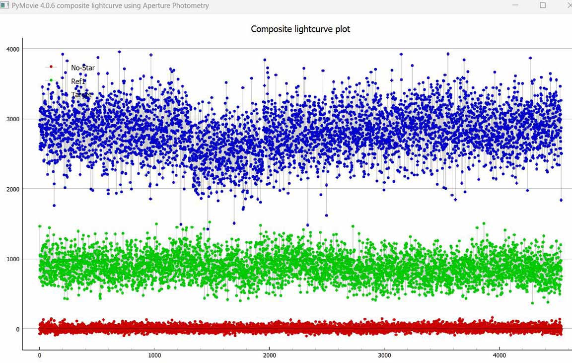
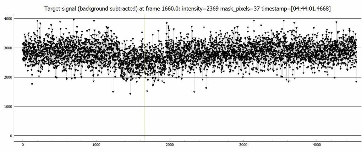
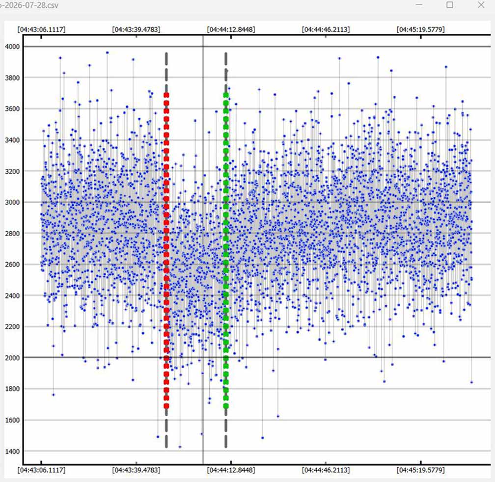
This analysis was a bit unusual. The ref star was much fainter than the target, and the target had some saturated pixels. Perhaps this was the cause of the fact that the raw data shows a well-behaved light curve, but after calibrating in PyOTE on the ref star, there was large oscillations in the target that were not present in the raw data, and this caused the first attempt to find the small drop D and R to be much longer than actual 31s instead of the far more likely 20-21s that nearby chords from Kirk Bender and I found. I suggested instead that Karl not use the reference star at all, and just run the PyOTE analysis on the uncalibrated PyMovie .csv file. The results are shown above, in good agreement with nearby chords. Karl's experience was the opposite of mine. For me, the reference star was essential to detect the occultation. For Karl, the reference star was fatal to the occultation proper detection. It pays to be careful.
This event brought back memories of my first asteroid occultation - of Juno - back on Dec 11, 1979 as a new PhD student at UCLA. I organized a group of grad students to drive out to near Castaic Junction, at Oak Flats NW of Los Angeles, and recorded the occultation by Juno with visual WWV/tape recorder old technology. Meanwhile, back at the rooftop observatory of the Astronomy building at UCLA, Dan McKenna led the photoelectric detection of the occultation. This was a well observed event, one of the best for asteroids at that time, and published in the AAS Journal PDF